Light-sheet 3D microprinting via two-colour two-step absorption

Two-colour two-step photoinitiation

The key ingredient of the photoresin is the photoinitiator. Upon absorption of light of wavelength λ₁, it enters an idle intermediate electronic state, from which the photoinitiator naturally decays back into its ground state. However, if the pre-excited idle photoinitiator absorbs a photon of wavelength λ₂, the molecule is further excited to an energetically higher state from which the polymerization reaction is initiated. The polymerization reaction crosslinks the liquid monomer, for example, by photoinitiator molecules fragmenting into free radicals. We refer to this process as two-colour two-step absorption. It is illustrated by an electron state diagram (Fig. 1c). Importantly, continuous-wave lasers can be used for both colours.

A good photoinitiator for light-sheet 3D printing must fulfil several criteria. First and foremost, one wants to avoid the case that light of either wavelength, λ₁ or λ₂, alone is able to promote both transitions in the photoinitiator and thereby triggering the polymerization reaction, which would result in an undesired crosslinking of the photoresin. Therefore, it is vital that the two-step absorption spectra of the ground and intermediate state contain non-overlapping regions (that is, the transitions are not degenerate). The two wavelengths are chosen such that the photoinitiator in its ground (intermediate) state does not absorb light of wavelength λ₂ (λ₁). Note that this choice is the polar opposite of what we have used in laser-scanning one-colour two-step absorption 3D nanoprinting²⁰, where one wavelength is intentionally chosen to trigger both optical transitions.

However, this criterion alone is not sufficient for a good two-colour two-step photoinitiator. A second crucial condition is that the photoinitiator molecule in its intermediate state decays back to the ground state in due time. Suppose this criterion is not fulfilled: after exposure of the first layer, the photoinitiator molecules along the entire optical path are promoted by light at wavelength λ₁ to the intermediate state—and remain there, even after progressing with the exposure to the next layer. In this layer, exposure with the light-sheet (at wavelength λ₂) alone suffices to polymerize the previous slice pattern in the photoresin. Hence, when exposing subsequent layers, one has to wait for the pre-excited photoinitiator molecules of the previously exposed layer to decay back to the ground state. This waiting time is governed by the intermediate-state lifetime and ultimately limits either the achievable printing rate or the spatial resolution.

The third criterion may appear somewhat counterintuitive at first sight. The photoinitiator’s ground-state extinction coefficient at wavelength λ₁ must be sufficiently low, such that a large enough intensity is transmitted to the focal plane. For example, typical photoresins contain photoinitiator concentrations in the range of 1% (wt.%) or about 20 mM (assuming a photoinitiator molar weight of 500 g mol⁻¹ and a mass density of 1 g ml⁻¹). Furthermore, assuming a molar decadic extinction coefficient of 1,000 M⁻¹ cm⁻¹ and a free-working distance of the projecting microscope objective lens of 500 μm, the light intensity would decay by an order of magnitude to 10% of the incident intensity via Beer’s law, which is clearly not acceptable.

Biacetyl and TEMPO as the photoinitiator system

A photoinitiator molecule that fulfils these three criteria is 2,3-butanedione, commonly known as diacetyl or biacetyl (Fig. 1b, top). A corresponding Jablonski diagram for biacetyl is shown in Fig. 1c. Upon absorption of a blue photon, the molecule is excited from the singlet ground state S₀ to an excited state S₁ and undergoes efficient intersystem crossing (99.8% quantum yield) to the triplet ground state T₁ (ref. ²¹). Biacetyl’s triplet ground-state energy of 235 kJ mol⁻¹ (2.44 eV) is relatively low^22,23,24 compared with other photoinitiators²⁵ and lower than typical bond-cleavage energies of 293 kJ mol⁻¹ (ref. ²⁶). Hence, biacetyl cannot efficiently fragment into radicals from its T₁ state. However, starting from the T₁ state, using light in the UV, red, and near-infrared regions²⁶, biacetyl can be optically excited to energetically higher states. The corresponding excited-state absorption spectrum is also plotted in Fig. 1d. In the excited triplet state, biacetyl has sufficient energy to fragment into radicals.

For all our experiments, we choose λ₁ = 440 nm. For the point-scanning pre-experiments, we use λ₂ = 640 nm (unless stated otherwise); for the light-sheet 3D printing experiments, λ₂ = 660 nm, where high-power solid-state laser sources are readily available. As evident from Fig. 1d, there is no overlap in the absorption spectra at the pair of wavelengths (λ₁ and λ₂) and hence the first criterion for a good light-sheet photoinitiator is fulfilled. The intermediate-state lifetime, that is, the triplet state in the case of biacetyl, was measured in degassed solutions and is on the order of 100 μs (ref. ²⁷), equivalent to a decay rate of 10⁴ s⁻¹. Since this rate is faster than the frame rate of available projectors and thus does not restrict the printing rate, the second criterion is met, too. Moreover, ingredients within the photoresin can act as a triplet quencher and further reduce the triplet lifetime^28,29,30,31. We will address the intermediate-state lifetime in the photoresin below, by comparison of the experimental data with rate equation calculations. Finally, at λ₁ = 440 nm, the molar decadic extinction coefficient in acetonitrile is 18 M⁻¹ cm⁻¹. With the used photoinitiator concentration of 110 mM and a microscope-lens free-working distance of 500 μm, the intensity in the focal plane only decays to about 80% of the incident intensity. Therefore, biacetyl also fulfils the third criterion.

However, similar to most ketones²⁴, biacetyl in its triplet ground state can abstract a hydrogen atom from nearby susceptible groups²⁴. Furthermore, thermally activated bond cleavage³² and reactions with oxygen³³ are possible decay mechanisms. These reactions potentially result in radicals being formed from the intermediate state. This behaviour is clearly undesired, as it would lead to the polymerization of photoresin triggered by light of only one wavelength, that is, λ₁. To suppress such unwanted side reactions, we introduce (2,2,6,6-tetramethylpiperidin-1-yl)oxyl (TEMPO) to the photoresin (Fig. 1b, bottom). TEMPO is a persistent radical and belongs to the group of hindered amine light stabilizers³⁴. It acts as a radical scavenger³⁵ and serves as a triplet-state quencher³⁰. In our experiments, we found that TEMPO efficiently suppresses polymerization triggered by only light of wavelength λ₁ under suitable conditions. We now quantify this aspect.

For our characterization experiments, we used three different photoresins PR1–PR3 (Table 1). The photoresins contain acrylate monomers of different viscosities and degrees of functionalization. We measured the polymerization threshold laser intensity of the photoresins by co-focusing two laser beams of wavelength λ₁ = 440 nm (blue) and λ₂ = 640 nm (red) through a large-numerical-aperture (NA = 1.4) objective lens into the photoresin and printing dashed-line patterns at a constant focus velocity of v₀ = 100 μm s^–1. The blue and red laser intensities are independently varied. For each red laser intensity I₂, we record the minimal blue laser intensity I₁ that leads to an optically visible polymerized line after sample development. This point marks the polymerization threshold. In Fig. 2a, we plot I₁ versus I₂ in a two-colour polymerization-threshold diagram on a double-logarithmic scale. On the right-hand-side vertical axis (Fig. 2b), the blue laser intensity is converted to blue power by using the measured full-width at half-maximum of the focus diameter of the blue laser. On the upper horizontal axis (Fig. 2b), the corresponding power for the red laser is given, similarly obtained from the full-width at half-maximum of the focus diameter of the red laser. The intensity scales allow for a direct comparison with the below light-sheet printing experiments. As evident from the figure, for zero and low red laser powers, the blue-laser threshold power is around P₁(P₂ = 0 mW) = 0.9 mW (corresponding to an intensity of 31 mW μm⁻²) for photoresin PR1. With increasing red laser power, the blue-laser polymerization threshold decreases in a sigmoid fashion and plateaus at about P₁(P₂ = 20 mW) = 4.6 μW (corresponding to an intensity of 0.16 mW μm⁻²). Hence, the two-colour polymerization contrast, which we define as the ratio of the two blue-laser threshold powers, is as large as about 200, consistent with the expectation for a good two-colour two-step absorption process. Ideally, this ratio should be infinitely large. The measured polymerization threshold intensities are in good agreement with the results of rate equation calculations (Fig. 2b). The rate model with an intermediate-state lifetime of <200 μs is discussed in detail in Supplementary Note 1.

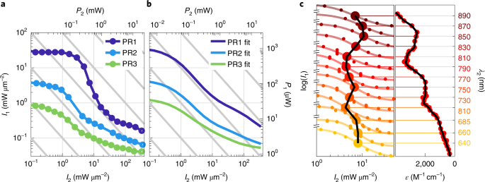
a, Two-colour point-scanning-exposure polymerization threshold experiments for three different photoresins (PR1–PR3), containing monomers of different viscosities. For increasing red laser intensity (I₂), the necessary blue laser intensity (I₁), at which the monomer is sufficiently crosslinked to form a solid polymer network, decreases. This effect is the most pronounced for the least viscous monomer, namely, trimethylolpropane triacrylate (TMPTA). Additional results of the point-scanning experiments are shown in Supplementary Figs. 6–8. b, Results of rate model calculations corresponding to the experiments shown in a. The curves qualitatively reproduce the experimental observations. Details on the calculations are provided in Supplementary Note 1. c, Stacked plot of two-colour point-scanning exposure experiments for photoresin PR1 using different red laser wavelengths λ₂. A logistic function is fitted to each experiment (not all the fitted data points fall within the plotted range). The sigmoid midpoint values are highlighted and outlined by the black curve. This curve can be compared with the triplet–triplet absorption spectrum of biacetyl (right). The triplet–triplet absorption data are extracted from elsewhere²⁶ (Fig. 1d). The black curve in c (right) is a smoothing spline curve through the red data points.

To further test the two-colour two-step absorption behaviour, we repeated the threshold power experiments for a set of red laser wavelengths λ₂, ranging from 640 to 890 nm. Figure 2c (left) shows the corresponding vertically stacked two-colour polymerization threshold data. Again, the data describe a sigmoid shape for all wavelengths λ₂ in the probed range. The solid curves are derived from fitting logistic functions to the measured data. The sigmoid midpoints are highlighted by a large dot and connected by a black curve. We expect the sigmoid’s midpoint location to correlate with the intermediate-state absorbance at the respective wavelength. Indeed, the two-colour two-step absorption character of biacetyl is confirmed by the black curve, that is, the action spectrum³⁶, which contains the characteristic minima and maxima of the extinction spectrum²⁶ (Fig. 2c, right). The detailed shapes of extinction and action spectra do not agree though, which points to not-well-understood aspects of photopolymerization in many systems beyond two-colour two-step absorption³⁶.

Light-sheet 3D printing setup

We now turn our attention to the actual light-sheet 3D printing experiments. For this purpose, a separate, dedicated setup was built. A diagram of the setup employed for light-sheet 3D printing is shown in Fig. 3a. It consists of two laser beam paths: one is the stationary red-light-sheet beam and the other one projects slices of the object using blue light. Both beams cross each other inside a cuboid cuvette chamber, which is mounted on a thin glass coverslip (Methods). The projection beam path consists of four multimode laser diodes. As evident from the emission spectra (Supplementary Fig. 3), the measured emission wavelengths scatter at around 440 nm. The diode’s spatial emission profiles are homogenized through a rectangular-core glass fibre. The fibre end facet is imaged onto a 720 Hz frame rate, high-definition liquid-crystal display (LCD), which is imaged through a long-working-distance, high-NA microscope objective lens into the cuvette. For the light-sheet beam, a 660 nm laser beam is shaped using a Powell lens into a line-shaped beam. This beam is then focused into the cuvette by a second microscope lens with low NA. Supplementary Notes 2 and 3 discuss the results of the light-sheet beam and projection beam characterization.

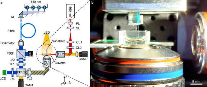
a, Sketch of the light-sheet 3D printing setup. AL, aspheric lens; PBS, polarizing beamsplitter; BD, beam dump; TL, tube lens; LCD, liquid-crystal display; CAM, camera; OL, objective lens; LED, light-emitting diode; CL, cylindrical lens; SL, spherical lens; PL, Powell lens. The detailed component lists are provided in the Methods section and Supplementary Tables 2 and 3. b, Photograph of the 3D printing glass-rod substrate, dipped into the cuvette. Below the cuvette, the projection objective lens is mounted. On the right-hand side, the light-sheet microscope objective lens can be seen.

A photograph of the mounted photoresin cuvette is shown in Fig. 3b. A glass rod of 1 mm diameter is dipped into the photoresin and the two objective lenses are focused onto the polished glass rod’s end facet, which serves as the 3D printing substrate. The glass rod is mounted on a set of precision translation stages (not depicted), including a low-inertia piezo-stage. By printing on a movable substrate, the printed structure dimensions are not limited by the field of view of the projected image. After printing, all the structures are developed for 30 s in acetone, with the exception of line gratings, which are supercritically dried in CO₂. In contrast to many other optical 3D printing methods, no laborious post-exposure UV illumination or other post-processing is necessary.

Voxel size and 3D printing rate

We determine the attainable minimum feature sizes of our light-sheet 3D printer by printing suspended line gratings with a length of 20 μm, pitch of 6 μm and fixed blue-laser exposure time of 5 ms (Fig. 4a). For this experiment, the red laser power is set to P₂ = 3 W, leading to a peak intensity of 3 mW μm⁻². The blue laser intensity in the focal plane is I₁ = 162 μW μm⁻². A plot of the measured linewidths versus the designed linewidths is shown in Fig. 4b. The smaller pale symbols indicate individual measurements, and the larger symbols are average values. The minimum reproducibly attainable linewidth and hence the voxel diameter is d_voxel = 0.5 μm, obtained for a projected linewidth of 9 pixels. However, the targeted linewidth in this case is 0.75 μm and hence larger. The ratio of targeted linewidth and measured linewidth decreases for wider lines. We attribute the deviation between attained and targeted linewidths to three aspects. First, the limited modulation transfer function of the projection system smears out the ideally rectangular illumination profiles (Supplementary Fig. 17). This rounding of exposure together with a threshold behaviour of the photoresin leads to a reduced linewidth. Second, before the monomer is crosslinked, quenchers and scavengers within the printing volume must be depleted^37,38. The depletion process proceeds faster in the centre of the printing volume than in the periphery, where the concentration of quenchers and scavengers is restored by an in-diffusion process from the unexposed surrounding (Supplementary Note 1). Third, polymer shrinkage may also contribute to the attained smaller linewidth. The corresponding line height is plotted on the right vertical scale (Fig. 4b). Evidently, a height of h_voxel = 2.2 μm is reproducibly achieved, resulting in a voxel aspect ratio of h_voxel/d_voxel = 4.4. We emphasize that it is possible to print even thinner lines. However, 32% of the six-pixel-wide lines broke during printing or development, which is contrasted by the 100% yield for the nine-pixel-wide lines. Hence, in the spirit of making conservative claims, we do not quote these values.

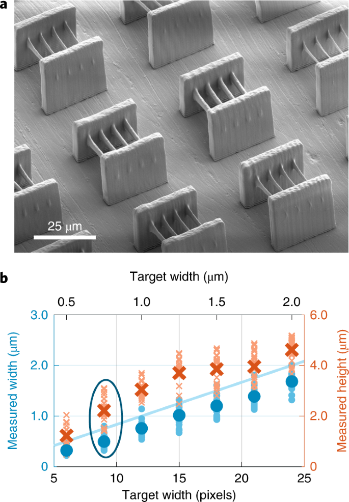
a, SEM image of a series of suspended lines with a pitch of 6 μm and length of 20 μm. The exposure time for each line grating was fixed at 5 ms. The blue laser intensity in the focal plane was I₁ = 160 μW μm⁻², and the red laser power was set to P₂ = 3 W to avoid possible saturation effects. During the exposure of lines, all the stages remained stationary. The grooved substrate surface is caused by the manual polishing process (Methods). b, Diagram of the measured linewidths (blue dots, left vertical axis) and measured line heights (red crosses, right vertical axis) versus the projected linewidth in units of pixels (bottom horizontal axis) or micrometres (top horizontal axis). The small dots (crosses) represent individual measurements and the large dots (crosses) indicate the average width (height). The measured linewidth increases monotonically with the projected width. The height increases monotonically and plateaus at a height of about 4 μm, which can be explained by the finite width of the incident light-sheet beam. We consider the encircled data points as the minimal reproducibly attainable voxel sizes.

On this basis, we derive the total peak voxel printing rate¹³. This metric allows for comparing different 3D printing approaches, which can have vastly different voxel volumes, in a meaningful manner¹³. The LCD has a resolution of 1,920 × 1,080 pixels, equivalent to a total of 2.07 × 10⁶ pixels. This value corresponds to 3.3 × 10⁴ voxels with the above voxel diameter of 9 pixels (assuming a round voxel shape). For an exposure time of 5 ms, as used for the printing of line gratings, we obtain a voxel printing rate of 7 × 10⁶ voxels s^–1 at a voxel volume of (0.5 μm)² × 2.2 μm = 0.55 μm³ and thus to a volume printing rate of 3.85 × 10⁶ μm³ s^–1. These values are compared with other 3D printing methods (Supplementary Fig. 20).

Light-sheet 3D printed structures

Scanning electron microscopy (SEM) images of 3D printed structures are shown in Fig. 5. We used the highly viscous photoresin PR3 for all the light-sheet 3D printed structures, since highly viscous multifunctional acrylates were found to have a long ‘intrinsic polymerization time constant’ and hence little change in refractive index occurs during the exposure phase³⁸. Therefore, scattering effects of the light-sheet at already polymerized parts are kept low. Figure 5a shows three knot-like structures, which were printed in parallel within 153 ms. Figure 5b shows a fleet of five #3DBenchy boats (https://www.laserchina.com/), which are a well-established benchmark structure in the community of 3D additive manufacturing. Each boat was printed within one printing field and took 266 ms to be printed. The boat’s hulls has a 100% filling fraction, resulting in proximity effects in the subsequent layers, that is, the boat’s window. To pre-compensate the proximity effect, we use a greyscale exposure profile, thus lowering the blue laser intensity in volumes with high local filling fraction (Supplementary Methods and Supplementary Fig. 19). In Fig. 5c, five quarter-cut acoustic metamaterial unit cells are printed on top of each other. This metamaterial was previously designed to yield a roton-like acoustic dispersion relation³⁹. The structure is especially challenging in fabrication using laser-scanning two-photon 3D microprinting: the outer walls are only fixed at two edges during printing, causing parts of the structure to drift off in the photoresin. For light-sheet 3D microprinting, this problem is absent, since each unit cell is printed within 117 ms. The entire stack is completed within 583 ms. The striped pattern on the structure’s surface is most probably the result of speckles arising from the blue beam path. The buckyballs (Fig. 5d) allow for a comparison with other 3D printing approaches^17,20. Each ball was printed within 250 ms. Finally, the chiral metamaterial⁴⁰ (Fig. 5e) has a footprint width of 155 μm, spanning almost the entire field of view. Despite the inhomogeneities observed in the light-sheet characterization (Supplementary Fig. 14), no irregularities are observed in the structure quality. Furthermore, the lattice constant of 77 μm is similar to our previously published study¹³. There, the printing time per unit cell was 1.6 s. Using light-sheet 3D microprinting, two unit cells were printed within 233 ms, that is, 117 ms per unit cell—a speedup of more than tenfold, although at a lower resolution. These structures prove that the presented photoresin and 3D printing setup are well suited for the fast production of 3D microstructures. However, we note that printing larger overall structures is still challenging for the used photoresin due to the gradual dose accumulation at the bottom of the photoresin vat, eventually leading to an impaired optical resolution for the projected layer.

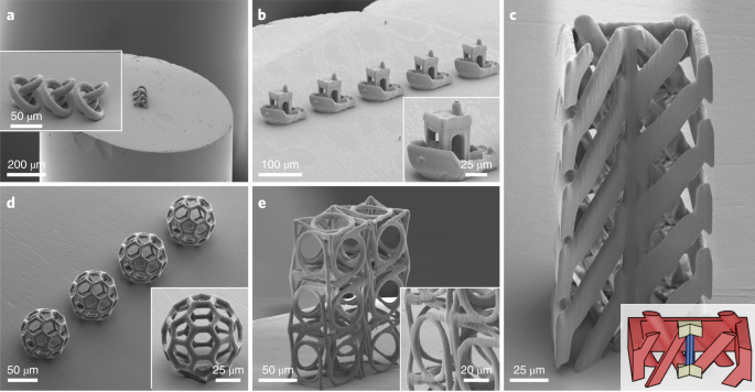
a, Knot-like structures printed on an intentionally slanted borosilicate glass rod. Three structures were printed in parallel. b, A small fleet of #3DBenchy structures. The inset reveals that overhanging features and holes are reproduced. The individual boats were sequentially printed by stitching several printing fields. c, Five stacked unit cells of a mechanical metamaterial, which was designed to obtain a roton-like acoustical-wave dispersion relation³⁹. The inset shows the rendering of a single unit cell from the same perspective. The large overhanging and flying features make this structure notoriously challenging to 3D print using laser-focus-scanning two-photon printing²⁹. A flyby SEM video is provided in the Supplementary Information. d, Buckyball structures with a diameter of 80 μm, sequentially printed by stitching several writing fields. e, Six chiral metamaterial unit cells⁴⁰. The inset reveals that the rings on the side walls are well separated from the adjacent vertically lying rings. The printing time per unit cell is 117 ms and hence more than ten times shorter compared with the results from a previous work employing laser-focus-scanning two-photon 3D nanoprinting¹³. All the 3D structures were printed at ~350 μm s^–1 substrate z velocity and blue-laser peak intensities of I₁ = 22 μW μm⁻². Real-time videos of the 3D printing process are available in the Supplementary Information.